
Geom
The Geom keyword specifies the source of the molecule specification input, options related to coordinate definitions, and geometry-related output. By default, it is read from the input stream, as described previously. Geom may be used to specify an alternate input source. It also controls what geometry-related information is printed and use of internal consistency checks on the Z-matrix. The Geom keyword is not meaningful without at least one item selection option.
By default, Gaussian uses generalized internal coordinates (GICs), a facility which automatically defines arbitrary redundant internal coordinates to be used for optimization constraints and other purposes [Marenich25]. The GIC Info subsection introduces using GICs.
Geometry Retrieval Options
Checkpoint
Take the molecule specification (including variables) from the checkpoint file. Only the charge and multiplicity are read from the input stream. For example, Geom=Checkpoint may be used by a later job step to retrieve the geometry optimized during an earlier job step from the checkpoint file. Checkpoint may be combined with the ModRedundant option or with the AddGIC option if you want to retrieve and alter the molecule specification in a checkpoint file using internal coordinate-style modifications. Note that Geom=(Checkpoint,ModRedundant,GIC) is equivalent to Geom=(Checkpoint, AddGIC). The Geom=(Checkpoint,GIC) option (i.e., without ModRedundant) will not use the GICs from the checkpoint file, but instead, it will build a new set of GICs automatically based on the current molecular specification (e.g., Cartesian coordinates) from the checkpoint file. The Geom=(Checkpoint,ReadAllGIC) option will not use the GICs from the checkpoint file, but instead, it will read a new set of GICs from the input file and calculate their values based on the current molecular specification (e.g., Cartesian coordinates) from the checkpoint file. Note that Geom=(Checkpoint,GIC) is equivalent to Geom=Checkpoint Opt=GIC, and Geom=(Checkpoint, ReadAllGIC) is equivalent to Geom=Checkpoint Opt=ReadAllGIC.
AllCheck
Take the molecule specification (including variables), the charge and multiplicity, and the title section from the checkpoint file. Thus, only the route section and any input required by keywords within it need be specified when using this option. This option is not valid with Modify but may be combined with ModRedundant, GIC, or AddGIC in the same way as the Checkpoint option.
Input
The source from which to retrieve each required geometry will be specified on a line in the input file. The title section and charge and multiplicity are included in the input file as normal, and the location from which to obtain the (first) structure follows the latter. Note that the title and charge and spin are not repeated for any subsequent geometries. The location can be specified as:
- The path to a checkpoint file (including the file extension).
- The form i from chk-name where i is the number of the intermediate structure from an optimization, dynamics calculation, IRC, etc. For example, ot=10 from lowopt.chk retrieves the tenth intermediate structure from the specified checkpoint file. i can also be a range of structures: e.g., 3-8. ot is replaced by relax when retrieving optimized structures from a previous relaxed scan calculation. For IRC calculations, ot uses the structure numbering following the order in which the points were computed; use irctab instead to specify structures using the numbering in the summary table at the conclusion of the output. You can also use the forms forward=n and reverse=n to specify the nth structure from the transition state in the indicated direction, and ts to retrieve the transition structure itself.
- The literal value zmatrix, which says to read a normal molecule specification immediately following in the input file (blank line terminiated as usual).
The form AllInput reads the title section and charge and multiplicity from the source of the first structure and uses them for all subsequent structures (if any).
NoReadInternal
Do not retrieve internal coordinates when retrieving a geometry from a checkpoint file. NoRdInternal is a synonym.
Step=N
This option retrieves the structure produced by the Nth step of a failed or partial geometry optimization (it is not valid for a successful optimization). Step=Original recovers the initial starting geometry. This option is used for restarting geometry optimization from intermediate points. It must be combined with one of Checkpoint, AllCheck, or Modify. Note that not all steps are always present in the checkpoint file; a Hessian updated message in the log file means that the corresponding step is available in the checkpoint file. NGeom=N retrieves the Nth geometry from an optimization checkpoint file using the same record of points used for display in GaussView, where N=1 corresponds to the input molecule specification. Geom=Step=M is automatically converted to Geom=NGeom=M+1 if the previous optimization used redundant internal coordinates.
Modify
Note that this option refers to modification specifications for geometry optimizations using Z-matrix coordinates only. In general, it is deprecated in favor of ModRedundant. It should not be used with GICs. Use Geom=(Checkpoint,AddGIC) instead of Geom=Modify if you want to modify the generalized internal coordinates.
This option specifies that the geometry is to be taken from the checkpoint file and that modifications will be made to it. A total of two input sections will be read: the first contains the charge and multiplicity, and the second contains alterations to the retrieved geometry.
Modification specifications for geometry optimizations using Z-matrix coordinates have the following form:
variable [new-value] [A|F|D]
where variable is the name of a variable in the molecule specification, new-value is an optional new value to be assigned to it, and the final item is a one-letter code indicating whether the variable is to be active (i.e., optimized) or frozen; the code letter D requests numerical differentiation be performed with respect to that variable and activates the variable automatically. If the code letter is omitted, then the variable’s status remains the same as it was in the original molecule specification.
Specifying Connectivity
Connectivity
Specify explicit atom bonding data via an additional input section (blank line-terminated) following the geometry specification and any modification to it. This option requires one line of input per atom, ordered the same as in the molecule specification, using the following syntax:
M N1 Order1 [N2 Order2 …]
where M is the atom number, the ‘N‘s are atoms to which the current atom is bonded, and the ‘Order‘s are the bond order of the corresponding bond. For example, this input specifies that the current atom is bonded to atoms 4 and 5, with bond orders of 1.0 and 2.0 respectively:
8 4 1.0 5 2.0
A bond order of 0.1 indicates a bond which should be used in generating internal coordinates but which should not affect atom types or connectivity for molecular mechanics.
This input section is terminated by a blank line.
ModConnectivity
Modify the connectivity of the atoms in the molecule specification (or retrieved from the checkpoint file). This option requires an additional input section (blank line-terminated) following the geometry specification and any modification to it. Connectivity modifications use the following syntax:
M N1 Order1 [N2 Order2 …]
where M is the atom number, the ‘N‘s are atoms to which that atom is bonded, and the ‘Order‘s are the bond order of the corresponding bond. A bond order of -1.0 removes a bond. For example, this input specifies that atom 8 is bonded to atoms 4 and 5, with bond orders of 1.0 and 2.0 respectively, and removes any bond to atom 9:
8 4 1.0 5 2.0 9 -1
This input section is terminated by a blank line.
GenConnectivity
Recompute connectivity rather than using the information in the checkpoint file when using Geom=AllCheck.
ZMConnectivity
Read connectivity using the atom numbering specified in the Z-matrix (including dummy atoms). Bond orders involving dummy atoms are discarded.
Fragment-related Options
ReadFragments
Read an input section listing the atoms in each fragment, with fragments separated by a forward slash character.
NoDefaultFrag
If no fragment information is provided in the molecule specification, then do not generate defaults based on the connectivity. NoDefFrag is a synonym.
Applying Harmonic Constraints
IHarmonic=n
Add harmonic constraints to the initial structure with force constant n/1000000 Hartree/Bohr2. InitialHarmonic is a synonym for this option.
ChkHarmonic=n
Add harmonic constraints to the initial structure saved on the checkpoint file with force constant n/1000000 Hartree/Bohr2. CHarmonic is a synonym for this option.
ReadHarmonic=n
Add harmonic constraints to an additional structure read in the input stream (in the input orientation), with force constant n/1000000 Hartree/Bohr2. RHarmonic is a synonym for this option.
Specifying the List of Atoms to be Optimized
ReadOptimize
Read an input section modifying which atoms are to be optimized. The atom list is specified in a separate input section (terminated by a blank line). By default, the atom list contains all atoms in the molecule, unless any atoms are designated as frozen within the molecule specification, in which case the initial atom list excludes them. If the structure is being read in from the checkpoint file, then the list of atoms to be optimized matches that in the checkpoint file. ReadOpt and RdOpt are synonyms for this option. ReadFreeze and RdFreeze are deprecated synonyms.
The input section uses the following format:
atoms=list [notatoms=list]
where each list is a comma- or space-separated list of atom numbers, atom number ranges, and/or atom types. Keywords are applied in succession. Here are some examples:
| atoms=3-6,17 notatoms=5 | Adds atoms 3,4,6,17 to atom list. Removes 5 if present. |
| atoms=3 C 18-30 notatoms=H | Adds all C & non-H among atoms 3, 18-30. |
| atoms=C N notatoms=5 | Adds all C and N atoms except atom 5. |
| atoms=1-5 notatoms=H atoms=8-10 | Adds atoms 8-10 and non-hydrogens among atoms 1-5, |
Bare integers without a keyword are interpreted as atom numbers:
| 1,3,5 7 | Adds atoms 1, 3, 5 and 7. |
You can start from an empty atom list by placing noatoms as the first item in the input section. For example, the following input optimizes all non-hydrogen atoms within atoms 1-100 and freezes all other atoms in the molecule:
noatoms atoms=1-100 notatoms=H
The keyword allatoms similarly specifies all atoms within the molecule.
For ONIOM optimizations only, block and notblock can be similarly used to include/not include rigid blocks defined in ONIOM molecule specifications. If there are contradictions between atoms specified as atoms and within blocks—e.g., an atom is included within a block but excluded by atom type—Gaussian generates an error.
Atoms can also be specified by ONIOM layer via the [not]layer keywords, which accept these values: real for the real system, model for the model system in a 2-layer ONIOM, middle for the middle layer in a 3-layer ONIOM, and small for the model layer of a 3-layer ONIOM. Atoms may be similarly included/excluded by residue with residue and notresidue, which accept lists of residue names. Both keyword pairs function as shorthand forms for atom lists.
Micro
Set up redundant internal coordinates for ONIOM(MO:MM) microiterations, even if this is not an optimization.
Output-Related Options
Distance
This option requests printing of the atomic distance matrix (which is the default for molecules with fewer than 50 atoms). NoDistance suppresses this output.
CAngle
This option requests printing of interatomic angles using distance cutoffs to determine “bonded atoms”. The default is not to print (NoAngle). Angle requests printing of the interatomic angles for Opt=Z-matrix (using the Z-matrix to determine which atoms are bonded). Only one of CAngle, Angle, and NoAngle may be specified.
CDihedral
This option requests printing of dihedral angles using distance cutoffs to determine “connectivity”. The default is not to print (NoDihedral). Dihedral specifies printing of dihedral angles for Opt=Z-matrix (using connectivity information from the Z-matrix to decide which atoms are bonded). Only one of CDihedral, Dihedral, and NoDihedral may be specified.
PrintInputOrient
This option includes the table giving the Cartesian coordinates in the input orientation within the output file.
This option turns on additional printing by the model builder facility.
Quiet
Suppress NAtoms length output to reduce output file size when running many geometries.
Geometry Checking Options
Crowd
Crowd activates and NoCrowd turns off a check that aborts the job if atoms are closer than 0.5 Å. By default, the check is performed for every read-in geometry. It is not performed by default for later points of geometry optimizations, numerical frequencies, etc., when the geometry has been generated during the job. NoTest skips the test entirely.
Independent
Independent activates and NoIndependent turns off a check on the linear independence of the variables specified in a Z-matrix. This is done by default only if a full optimization is requested using the Berny algorithm (Opt=Z-matrix).
Other Options
Huge
Changes various defaults for huge (>20K atom) systems. Currently, this sets Geom=NoTest and Symm=None.
Generalized Internal Coordinate (GIC)-Related Options
The options that do not mention GIC and can be used with the Geom keyword should work as described—except for NewDefinition and NewRedundant. The latter should not be combined with any GIC-related option. In the case of GICs, you should use Geom=(Checkpoint,GIC) instead of Geom=NewDefinition, Geom=GIC instead of Geom=NewRedundant, and Geom=(Checkpoint,addGIC) instead of Geom=(Modify,NewRedundant).
See General Internal Coordinates for more information on GICs.
GIC
Build an automatic set of redundant internal coordinates using the new GIC algorithm. Geom=GIC is now equivalent to Geom=Redundant and the default is to use GICs whenever the internal coordinates are requested. The coordinates generated with this option can be the same bonds, angles, and dihedral angles generated using the old algorithm [Peng96] if the input geometry does not have any disjoint fragments that require a special treatment with the option Geom=(GIC,Rotors) or any methyl or similar XY3-type functional groups attached to the main skeleton that require a special treatment with the option Geom=(GIC,XY3) (see below). With a few exceptions noted below, Geom=(GIC,Rotors,XY3) is used by default. The option Geom=(GIC, NoRotors,NoXY3) can be used to build only regular bonds, valence angles, and dihedral angles and to use virtual bonds in case if there are disjoint fragments. Opt=GIC can be used as well. If Opt is requested, perform the optimization using the Berny algorithm with the GICs.
DefNoGIC
Build an automatic set of redundant internal coordinates such as bonds, angles, and dihedrals from the current Cartesian coordinates or Z-matrix values using the old algorithm (Peng96) available in Gaussian 16 (no GICs). Opt along with Geom=DefNoGIC can be used as well. If Opt is requested, perform the optimization using the Berny algorithm in these redundant internal coordinates. This was the old default in Gaussian 16.
AddGIC
Build the same GICs as described above. Then read the input stream for user-provided modifications to those GICs before performing any further calculation. This option requires a separate input section following the geometry specification. The syntax of the GIC input section is described in GIC SYMBOLIC INPUT DICTIONARY. The option Opt=AddGIC can be used as well. The option Geom=(GIC,ModRedundant) and Geom=ModRedundant are equivalent to Geom=AddGIC. The option Geom=(DefNoGIC,ModRed) can be used to request the old redundant coordinates [Peng96] modified according to the old modred input. ModRed and ModRedundant are equivalent.
ReadAllGIC
Do not build any redundant internal coordinates by default. Instead, read the input stream for user-provided GIC definitions and create the coordinates. This option requires a separate GIC input section following the geometry specification. The syntax of the GIC input section is described in GIC SYMBOLIC INPUT DICTIONARY. The default is Geom=(ReadAllGIC,NoRotors,NoXY3). The option Opt=ReadAllGIC can be used as well.
ChkGIC
Read all GICs from the checkpoint file and apply them to the current input Cartesian geometry.
GICOneSymm
Form symmetry combinations of the GICs for the totally symmetric irreproducible representation (replacing original GICs).
GICAllSymm
Form symmetry combinations of the GICs and retain all irreproducible representations (replacing original GICs).
GICAllFSymm
Form symmetry combinations of the GICs, retain all irreducible representations, and freeze all the combinations except the totally symmetric ones (replacing original GICs).
GICOld
Build an automatic set of redundant internal coordinates using the old algorithm (Peng96), read the old modred input in the case of Geom=ModGICOld, and then convert the coordinates into the GICs and treat them as such. No other options such as Rotors or XY3 can be used here. Use this option for the old algorithm input cases that do not work with the new GIC code without input modification.
GICZMatrix
Read regular Z-matrix coordinates from the input and then convert them into GIC-type internal coordinates with the original Z-matrix constraints being preserved. The option Opt=GICZmat is acceptable as well. If Opt is requested, perform a geometry optimization like with Opt=Z-Matrix but in terms of the GICs. No other options such as Rotors or XY3 can be used here. To find the corresponding input examples, run the following command:
grep -i 'GICZmat' $gdvroot/gdv/tests/com/*.com
Build the GIC-type Z-matrix coordinates and constraints (as described above) and then read the input stream for user-provided modifications to those GICs before performing any further calculation. The syntax of the GIC input section is described in GIC SYMBOLIC INPUT DICTIONARY. The option Opt=(GICZmat,AddGIC) is acceptable as well.
Rotors
Build a special set of GICs (called below the fragment-based rotor-type GICs) to treat disjoint fragments determined from the input Cartesian geometry or from the user-provided connectivity information and do not build any virtual bonds between the fragments. The connectivity information can be introduced by using the option Geom=Connectivity. This is the default for Geom=GIC if two or more qualified fragments are detected. In particular, the fragments should have more than two atoms and this is for a regular calculation that does not use periodic boundary conditions (PBCs), ONIOM with micro-iterations, QST2, QST3, Path, Cartesian atoms or the RdOpt option. Otherwise, the default for Geom=GIC is Geom=(GIC,NoRotors).
The fragments can also be specified explicitly in the Cartesian input section like in the case of a counterpoise calculation request:
O(fragment=1)  0.000000000000      0.000000000000      0.000000000000
H(fragment=1)  0.000000000000      0.000000000000      0.976756085872
N(fragment=2)  0.259655068263      0.000000000000      2.877762253635
H(fragment=2)  1.269044288026      0.000000000000      2.982267037494
H(fragment=2) -0.089902960790      0.816744932713      3.367111592058
H(fragment=2) -0.089902960790     -0.816744932713      3.367111592058
H(fragment=1) -0.924602146888      0.000000000000     -0.254984428189
The current version of the code assigns the fragment-based rotor-type GICs automatically to any default or user-specified fragment used in a counterpoise calculation. If one wants to use regular bonds, valence and dihedral angles instead then the option Geom=(GIC,NoRotors) should be specified to override the Rotors default.
The fragment-based rotor-type GICs include the default internal coordinates (regular bonds, valence and dihedral angles) for individual fragments and an additional set of coordinates to describe the rotational and translational motion of each fragment. The translational GICs of fragment k with Nk atoms are the Cartesian coordinates of its center of geometry (labeled by default as Cxk , Cyk , and Czk ):
Cxk = ( ΣXik )/Nk
Cyk = ( ΣYik )/Nk
Czk = ( ΣZik )/Nk
where Σ means a sum over i and the index i runs over Nk atoms in the fragment defined by the atoms’ Cartesian coordinates. The rotational GICs are the Cartesian components of the unit vectors Pk , Qk , and Sk (labeled by default as Pxk , Pyk , Pzk , Qxk , Qyk , Qzk , Sxk , Syk , Szk ) to describe the three orthogonal axes of rotation. The vector Pk is directed from the center of geometry (Ck) towards the atom ( Ak,1 ) selected to be most distant from the center and symmetrically unique, if possible. Otherwise, the first qualified atom from the list of symmetrically equivalent ones will be used. The vector is defined by the three GICs:
Pxk = (X1k – Cxk )/R(1, Ck )
Pyk = (Y1k – Cxk )/R(1, Ck )
Pzk = (Z1k – Cxk )/R(1, Ck )
The direction of the unit vector Qk is defined by a vector product of the vector Pk and the vector spanning from Ck to the second atom ( Ak,2 ). The latter is selected to be a symmetrically unique atom (if possible) with the smallest absolute value for the dot product CkAk,1·CkAk,2 and it cannot be the one closest to the center of the fragment at the same time:
Q0xk = Pyk ( Z2k – Czk ) – Pzk ( Y2k – Cyk )
Q0yk = Pzk ( X2k – Cxk ) – Pxk ( Z2k – Czk )
Q0zk = Pxk ( Y2k – Cyk ) – Pyk ( X2k – Cxk )
RQ0k = ( Q0xk2 + Q0yk2 + Q0zk2 )1/2
Qxk = Q0xk / RQ0k
Qyk = Q0yk / RQ0k
Qzk = Q0zk / RQ0k
The vector Sk is the vector product Pk ⊗ Qk:
Sxk = Pyk Qzk – Pzk Qyk
Syk = Pzk Qxk – Pxk Qzk
Szk = Pxk Qyk – Pyk Qxk
An additional set of six GICs is introduced to freeze the total translations by freezing the center of geometry for the whole N-atom molecule at its initial position as
XTr(Frozen) = (ΣXi)/N
YTr(Frozen) = (ΣYi)/N
ZTr(Frozen) = (ΣZi)/N
and to freeze the total rotations with respect to the initial (reference) geometry as
XRot(Frozen) = (Σ[ Yi* Zi – Zi* Yi ])/N
YRot(Frozen) = (Σ[ Zi* Xi – Xi* Zi ])/N
ZRot(Frozen) = (Σ[ Xi* Yi – Yi* Xi ])/N
where Σ means a sum over i which runs over all the N atoms, and the asterisk refers to the initial values of Cartesian coordinates for atom i (to be determined automatically from the input geometry). This is equivalent to using the Eckart conditions for translations and rotations (see, for example, Page 210 in [Bunker, P. R.; Jensen, P. Molecular symmetry and spectroscopy, 2nd edition, NRC Research Press, Ottawa, 2006]) with all the atomic masses nominally equal to 1 a.u. The translation center of the whole molecule can be placed at the origin of the Cartesian coordinate system by means of IOp(1/156=2xxxx), if desired.
Note that in certain calculations (e.g., with fragments larger than 50 atoms and for some non-regular cases such as PBCs or ONIOM with microiterations) the fragment-based rotor-type GICs of the largest fragment k or, in case of ambiguity, the first largest fragment ( Cxk through Szk ) will not be built by default and the expressions XTr , YTr , ZTr , XRot , YRot , and ZRot introduced above will be used to freeze the total translations and rotations of that fragment instead of the whole molecule (the index i would run only over Nk atoms in the fragment).
In the case of linear fragments, the vectors Qk and Sk are undefined and their components are replaced with the Cartesian coordinates of the remaining atoms (after the first one). One-atom fragments (they are not assigned by default in the current code) are described using the corresponding Cartesian coordinates.
The option Opt=(GIC,Rotors) is acceptable as well. If Opt is requested, perform a geometry optimization using the resulting GICs. To find the corresponding input examples, run the following command:
grep -i Rotors $gdvroot/gdv/tests/com/*.com | grep -v -i NoRotors
QRotors
Build a special set of the fragment-based rotor-type GICs (to treat disjoint fragments as described above) labeled by default as Pxk , Pyk , Pzk , Qxk , Qyk , Qzk , Sxk , Syk , Szk along with the translation-type GICs labeled as Cxk , Cyk , and Czk for each fragment k and convert them into the quaternion GICs. The rotation (unit) quaternion for each fragment is defined as one scalar component (K0) and three vector components (K1 , K2 , K3 ) in terms of the 3×3 rotation matrix (see, for example, Page 169 in [Kuipers, J. B. Quaternions and rotation sequences: a primer with applications to orbits, aerospace, and virtual reality, Princeton University Press, 2002]) as follows:
K0 = (R11 + R22 + R33 + 1)1/2 / 2
K1 = (R23 − R32) / (4K0)
K2 = (R31 − R13) / (4K0)
K3 = (R12 − R21) / (4K0)
The rotation matrix in turn is expressed in terms of the dot products of the P, Q, and S vectors for the same fragment as follows:
| R11 = P·P* | R12 = P·Q* | R13 = P·S* |
| R21 = Q·P* | R22 = Q·Q* | R23 = Q·S* |
| R31 = S·P* | R32 = S·Q* | R33 = S·S* |
The P, Q, or S unit vectors are defined in terms of their Cartesian components at the current geometry (no asterisk) and at the initial geometry (with the asterisk). Thus, the rotation of a fragment is defined wrt its initial position around the center of geometry which can move independently.
The option Opt=(GIC,QRotors) is acceptable as well. If Opt is requested, perform a geometry optimization using the resulting GICs. To find the corresponding input examples, run the following command:
grep -i -e QRotors -e FlQua0 $gdvroot/gdv/tests/com/*.com
NoRotors
Do not build a special set of GICs to treat disjoint fragments even if there are such fragments. Use regular bonds, valence and dihedral angles as well as virtual bonds to connect the fragments, if any, or any coordinates that come from a user-provided GIC input section. Note that NoRotors is the default for Geom=GIC and AddGIC when used with PBCs, micro-iterative ONIOM, QST2 or similar options and it is always the default for Geom=ReadAllGIC.
NoDefaultFrag
Do not look into the default or user-provided connectivity data for any default fragments. Use regular and virtual bonds, valence and dihedral angles or any coordinates that come from a user-provided GIC input section. Note that a combination of NoDefaultFrag and Rotors with no user-provided fragment information in the GIC input section will cause an error.
XY3
Identify any methyl (CH3) or similar non-planar groups (XY3 or XYY’Y” in general) from the input geometry or connectivity. The connectivity information can be introduced by using the option Geom=(Connectivity,GIC). Build the default GICs (bonds, angles, and dihedral angles) for the remaining skeleton. Build a special set of GICs for the detected XY3-type groups (see the scheme on the right). This is the default for Geom=GIC for any molecule larger than neopentane (17 atoms) and this is for a regular calculation without PBCs, ONIOM with micro-iterations, QST2, QST3, Path, Cartesian atoms or the RdOpt option. Otherwise, the default for Geom=GIC is Geom=(GIC,NoXY3). The option Opt=(GIC,XY3) is acceptable as well. If Opt is requested, perform a geometry optimization using the resulting GICs. Note that the XY3 groups connected to the same atom Z as well as for some special cases (e.g., when some WZX or VWZ angles are linear) will not be assigned the XY3-type GICs automatically because the latter may not work better than regular coordinates. Use a special internal option (IOp(1/156=4x)) to override this restriction. The default label for the torsion GIC (T in the scheme) for each XY3 group is TOxI where I refers to the atomic index for atom X. The deformation GICs (DA and DB) are labeled as DAxI and DBxI. The remaining coordinates generated for each XY3 by default are pure bonds, valence angles, and dihedral angles (labeled as such).
Build a special set of GICs to treat the XY3-type groups as described above and then read an additional GIC input to modify the new GICs. Note that such groups must be present if the XY3 option is specified explicitly. The option Opt=(AddGIC,XY3) is acceptable as well. If Opt is requested, perform a geometry optimization using the resulting GICs. To find the corresponding input examples, run the following command:
grep -i XY3 $gdvroot/gdv/tests/com/*.com | grep -i -v NoXY3
Read the input stream for user-provided GIC definitions that should include the internal coordinates for the skeleton. Build a special set of GICs for the XY3-type groups detected automatically. Note that such groups must be present. The default is Geom=(ReadAllGIC,NoXY3). The option Opt=(ReadAllGIC, XY3) is acceptable as well. If Opt is requested, perform a geometry optimization using the resulting GICs. To find the corresponding input examples, run the following command:
grep -i XY3 $gdvroot/gdv/tests/com/*.com | grep -i ReadAllGIC
NoXY3
Do not build a special set of GICs to treat the XY3-type groups even if there are such groups. Use regular bonds, valence and dihedral angles or any coordinates that come from a user-provided GIC input section. Note that NoXY3 is the default for Geom=GIC and AddGIC when used with PBCs, micro-iterative ONIOM, QST2 or similar options and it is always the default for Geom=ReadAllGIC.
Symmetrized internal coordinates
GICAllSym
Build the default initial GICs as a set of regular bonds, valence and dihedral angles for the current input geometry and symmetrize them based on the current point group (determined from the input Cartesian coordinates) by building symmetrized linear combinations according to each irreducible representation. The option Opt=GICAllSym is acceptable as well. If Opt is requested, perform a geometry optimization using the symmetrized GICs. If the options Opt=QST2 or Opt=QST3 are used as well then the symmetrization will be applied to the final GICs generated for the union (transition state) structure. If there are no other automatic options such as Rotors or XY3 specified explicitly then the initial (unsymmetrized) GICs will be regular internal coordinates with disjoint fragments being connected by virtual bonds (if any) and with no special treatment of XY3-type functional groups (if any). The default is Geom=(GICAllSym,NoRotors, NoXY3).
GICAllFSym
Do Geom=GICAllSym but also freeze all the non-totally symmetric GICs. The option Opt=GICAllFSym is acceptable as well. If Opt is requested, perform a geometry optimization using the symmetrized GICs for the totally symmetric irrep (e.g., for A1g in Oh) with the remaining GICs being kept frozen to preserve the current symmetry. If the symmetry is not expected to change upon geometry optimization, GICOneSym (see below) should be used instead of GICAllFSym. The default is Geom=(GICAllFSym,NoRotors, NoXY3).
GICOneSym
Build symmetrized combinations of GICs only for one irreducible representation, in particular, for the totally symmetric irrep (e.g., for A1g in Oh ). The option Opt=GICOneSym is acceptable as well. If Opt is requested, perform a geometry optimization using the IOp(1/156=1xxx) settings and the GICs symmetrized only for the totally symmetric irrep. The default is Geom=(GICOneSym,NoRotors,NoXY3).
ChkGIC
Read check-point GICs and apply them to the current Cartesian geometry from the input (do not use check-point Cartesian coordinates).
GICPrint
Prints all the primitive (intermediate) expressions for the current GICs and their first and second derivatives with respect to Cartesian coordinates (if applicable) in the form of a symbolic algebra tree. Note that the log file can be very big. The same functionality is available with IOp(1/33=3) (for GDV only). One can also use Geom=(AddGIC,GICPrint), Geom=(ReadAllGIC, GICPrint), etc.
DefaultGIC
Make GICs the default (for use in a Default.Route file)
DefaultNoGIC
Make Peng internal coordinates the default (for use in a Default.Route, but this is the default anyway).
Note on QST2 and QST3 calculations with GIC, AddGIC, ReadAllGIC, and other GIC-related options
The QST2 calculation requires two geometry specifications as usual (one for the reactants and another for the products). The QST3 calculation requires three geometry specifications (for the reactants, for the products, and for the transition state). The options Opt=(QSTx,GIC) where x is equal to 2 or 3 do not require any additional GIC-related input. The union GICs will be built by merging the default GICs for each of the two (QST2) or three (QST3) structures. If the linear bends are required for any of those structures then they will be retained while the corresponding regular angles and dihedral angles will be removed because they may be undefined at certain geometries. The options Opt=(QSTx,ReadAllGIC) require two separate GIC inputs as the only source of GICs where the first input follows the geometry specification for the reactants and the second input follows the geometry specification for the products (no GIC input for the third structure is needed). The options Opt=(QSTx,AddGIC) require one GIC input after the last QSTx geometry specification to modify the final GICs generated by default for the union (transition state) geometry. The options Opt=(QSTx,AddGIC,Y) with Y to be replaced with another keyword such as GICOneSym, GICAllSym, Rotors, or XY3 (note that not every possible combination will be practical or has been tested so far) require the second GIC input to modify the final GICs obtained after an automatic modification (e.g., symmetrization) of the transition-state GICs. Any missing GIC input section that is otherwise required should be replaced with an extra blank line. Here is an example of the QST2 input when we need to modify the final set of GICs (by freezing something in this case):
# hf/3-21g opt=(QST2,AddGIC) nosymm

QST2 reactant

0 2
 C                  0.00000000    0.00000000    0.00000000
 H                  0.00000000    0.00000000    2.00000000
 H                  1.08000000    0.00000000    0.00000000
 H                 -0.54000000   -0.93530744    0.00000000
 H                 -0.54000000    0.93530744    0.00000000
 F                 -0.00000000    0.00000000    2.92000000

QST2 product

0 2
 C                  0.00000000    0.00000000    0.00000000
 H                  0.00000000    0.00000000    1.08000000
 H                  1.01817859    0.00000000   -0.36015602
 H                 -0.50908930   -0.88176853   -0.36015602
 H                 -0.50908930    0.88176853   -0.36015602
 F                 -0.00000000    0.00000000    3.08000000

L(1,2,6,3,-1) Frozen
L(1,2,6,3,-2) Frozen
Here is an input for the same transition state calculation using QST3:
# hf/3-21g opt=(QST3,AddGIC) nosymm

QST3 reactant

0 2
 C                  0.00000000    0.00000000    0.00000000
 H                  0.00000000    0.00000000    2.00000000
 H                  1.08000000    0.00000000    0.00000000
 H                 -0.54000000   -0.93530744    0.00000000
 H                 -0.54000000    0.93530744    0.00000000
 F                 -0.00000000    0.00000000    2.92000000

QST3 product

0 2
 C                  0.00000000    0.00000000    0.00000000
 H                  0.00000000    0.00000000    1.08000000
 H                  1.01817859    0.00000000   -0.36015602
 H                 -0.50908930   -0.88176853   -0.36015602
 H                 -0.50908930    0.88176853   -0.36015602
 F                 -0.00000000    0.00000000    3.08000000

QST3 transition state

0 2
 C                  0.00000000    0.00000000    0.00000000
 H                  0.00000000    0.00000000    1.25000000
 H                  1.06359237    0.00000000   -0.18754003
 H                 -0.53179619   -0.92109801   -0.18754003
 H                 -0.53179619    0.92109801   -0.18754003
 F                 -0.00000000    0.00000000    2.50000000

L(1,2,6,3,-1) Frozen
L(1,2,6,3,-2) Frozen
To find more input examples, run the following command:
grep -i 'QST' $gdvroot/gdv/tests/com/*.com | grep -i GIC
Note on IRC calculations with GIC-related options
The intrinsic reaction coordinate (IRC) calculation does not use any GICs but it is possible to compute and print the values of user-specified GICs along the IRC path, provided that the IRC=Report option is requested as well. Find some examples by running the following command:
grep -i 'IRC' $gdvroot/gdv/tests/com/*.com | grep -i GIC
Redundant Internal Coordinates Specification and Modification Options
ModRedundant
For redundant internal coordinates, the ModRedundant option will add, delete, or modify redundant internal coordinate definitions (including scan and constraint information) before performing the calculation. This option requires a separate input section following the geometry specification. AddRedundant is synonymous with ModRedundant.
This option may be used for job types other than optimizations. It may also be combined with NGeom, Check or AllCheck to retrieve and modify an internal coordinate definition from a checkpoint file.
When used with Check, or NGeom, two input sections will be read: the first contains the charge and multiplicity, and the second contains alterations to the retrieved internal coordinate definition. When combined with the AllCheck option, only the internal coordinate definition modifications input is needed.
See the Red. Int. Coords. tab for details.
NewDefinition
Generate a new set of redundant internal coordinates, replacing any that were in the checkpoint file. This option should not be used with GICs; use Geom=(Checkpoint,GIC) instead.
SkipAll
Do not generate any internal coordinates automatically. In the case of redundant internal coordinates based on the old algorithm available in Gaussian 09, all of the required coordinates must be explicitly specified in the ModRedundant input section. In the case of GIC-type internal coordinates based on the new GIC algorithm, you should use Geom=ReadAllGIC instead of this option.
SkipAng
Generates bonds but omits angles and dihedrals.
SkipDihedral
Suppresses the generation of dihedrals.
SkipHBond
Skips generation of hydrogen-bond coordinates.
KeepConstants
KeepConstants retains and NoKeepConstants discards information about frozen variables. The default is to retain them in symbolic form for the Berny algorithm and to discard them for older optimization algorithms (which don’t understand them anyway).
NewRedundant
Rebuilds the redundant internal coordinates from the current Cartesian coordinates. If used with Geom=Modify, the new modifications are appended to any earlier Opt=ModRedundant input before the coordinate system is updated. This option should not be used with GICs; use GIC or AddGIC instead (as appropriate).
Redundant
Build an automatic set of redundant internal coordinates such as bonds, angles, and dihedrals from the current Cartesian coordinates or Z-Matrix values, using the old algorithm available in Gaussian 09.
UseStandardOrientation
Use the coordinates in the standard orientation from the checkpoint file as the input orientation for the new job when using Geom=AllCheck.
UseInputOrientation
If a structure is taken from the checkpopint file from a job which did not include NoSymm, use the input orientation from the checkpoint file as the input orientation for the current job. This is the default except for IRC calculations.
General information
The GIC input section is separated from the earlier input by a blank line. It has one or more lines containing coordinate definitions, expressions or standalone options. The basic form of a coordinate definition is the following:
label(options)=expression
Note that options may also be placed following the expression without a label:
Expression Options
Here is a simple GIC input section for water illustrating some of the possible features:
R(1,2)		               !Define a bond coordinate between atom 1 and atom 2
Bond2=R[1,3]		   !Define another bond and name it Bond2
HOH(freeze)=A(2,1,3)  !Define the valence angle and keep it frozen during geometry optimization
For a geometry optimization, this input will result in the bond angle remaining fixed at its initial value and the two bond distances being optimized. Note that the line “A(2,1,3) Freeze” will be valid while the line “HOH=A(2,1,3) Freeze” will not. The text after the ! mark is just an optional comment.
Labels are user-assigned identifiers for the coordinates. They are not case sensitive. Labels may contain letters and numbers, but must begin with a letter. If no label is specified, a generic one will be assigned by the program. The default label for bonds will be R1, R2, …, Rn where n runs over all generated bonds (active, frozen, and inactive) in the order of appearance. In a similar fashion, the default labels for angles will be A1, A2, etc. and default labels for dihedral angles will be D1, D2, etc. The default label for a generic GIC without a user-provided label is Gi where i is the index of the corresponding GIC primitive in the whole GIC expression tree. The latter can be printed out using IOp(1/33=3) (for GDV only), if necessary for debugging (note that the log file may be very large). A parenthesized, comma-separated list of options can be included following the label, if desired.
Coordinates are defined by expressions. The simplest expressions identify a specific structural parameter such as a bond, for example, R(1,2) where the indexes refer to specific atoms. Note that an asterisk may be used as a wildcard for any atom number in certain situations and the dummy atoms specified by the dummy() function can also be used. A coordinate definition expression in general may include available mathematical functions (arccos, sqrt, etc.) and operations (“+”, “-“, “*”, “/”, “**2”, etc.), as well as the labels of previously defined coordinates (R1, R2, etc.). The expression may use parentheses, square brackets, or braces. All of them can be nested, but mixing the different types, e.g. {), is not permitted. The letters in the expression are not case sensitive. The expression should not begin with “+”, “*”, “/” but may begin with “-”. For example, the line “-R1+R2” is permitted and will be equivalent to “R2-R1”, and expressions such as “(-1.)*R1+R2”, “-1.*R1+R2”, “-2.*R(1,2)”, and “-(-R(1,2)+R(1,3))” are all valid.
List of available functions to specify geometry parameters
R(i,j)
Define a bond coordinate between atoms i and j. Synonyms: B(i,j), Bond(i,j), Stretch(I,j).
A(i,j,k)
Define a non-linear angle coordinate involving atoms i, j, and k where atom j is at the angle vertex. Synonyms: Angle(i,j,k), Bend(I,j,k).
D(i,j,k,l)
Define a dihedral angle between the plane containing atoms I, j, and k and the plane containing atoms j, k, and l. Synonyms: Dihedral(i,j,k,l), Torsion(I,j,k,l).
L(i,j,k,L,M)
Define the first (M = -1) or the second (M = -2) component of the linear bend coordinate involving atoms i, j, and k where atom j is at the angle vertex. The values of M other than -1 or -2 are not permitted. The L can be -4, -3, -2, -1, 0, or >0. A value of L = -4 or L > 0 is applicable only to a nonlinear molecule with more than three atoms. A value of L > 0 means that the linear bend between i, j, and k is specified using the 4th atom L which does not form a linear angle with i, j, and k in any combination. The 4th atom is used to build the two orthogonal directions of the linear bend (one for M = -1 and another for M = -2). If L = -4, the 4th atom will be determined by default based on the molecule’s geometry. The values L = 0, -1, -2, or -3 mean that the 4th atom is not used and the given component M is determined by projecting the linear bend onto the YZ, XZ, or XY plane in the case of L = -1, -2, -3, respectively, or onto any of these planes as determined by default if L = 0. The 3-atom linear bend is the only option for a linear molecule. Synonyms: Linear(i,j,k,L,M), LinearBend(I,j,k,L,M).
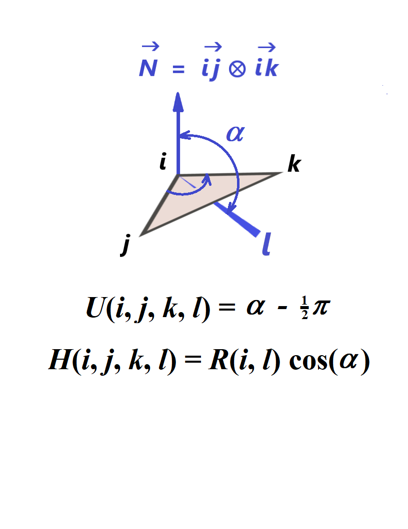
U(i,j,k,l)
Define an umbrella-type coordinate involving atoms i, j, k, and l as an angle formed by the i-l vector and the i-N vector minus 90º where i-N is the vector product of i-j and i-k. See the figure on the right. The coordinate changes from -90º to 90º.
H(i,j,k,l)
Define an umbrella-type coordinate involving atoms i, j, k, and l as a signed distance between the j-i-k plane and the atom l. See the same figure. The coordinate changes from -R(i,l) to R(i,l) where R(i,l) is the distance from i to l.
DotDiff(i,j,k,l)
Define the dot product (a·b) of the two Cartesian coordinate difference vectors a and b for atoms i, j, k, and l determined as a = (Xi – Xj, Yi – Yj, Zi – Zj) and b = (Xk – Xl, Yk – Yl, Zk – Zl). The values i, j, k, and l can be equal to any valid atomic center number.
Label=Dummy(X,Y,Z)
Define a GIC dummy atom along with some user-provided label (replace “Label” with the actual label) whose Cartesian coordinates are either functions of some previously defined GICs (X, Y, and Z should be replaced with actual labels for those GICs) or simply some points in space where X, Y, and Z are floating-point values in the units defined by the Units keyword (Angstroms by default). This GIC does not add any new coordinate and it is used as an intermediate expression to build other GICs. Find some examples of using GIC dummy atoms by running the following command:
grep -i 'Dummy(' $gdvroot/gdv/tests/com/*.com
Fragment(i–j)
Label=Fragment(i–j)
Define a molecular fragment along with an optional label (replace “Label” with the actual label) that contains specified atoms separated by commas or/and hyphens. The default labels are FRGM1, FRGM2, etc. For example, the interval (1,2-5,7) refers to atoms #1, 2, 3, 4, 5, and 7. Wildcards (asterisks) and dummy atoms are not permitted. To specify a fragment that extends to the whole molecule (for example, with 8 atoms) use the interval (1-8). This GIC does not add any new coordinate and it is used as an intermediate expression to build other GICs (see examples).
Label(Frozen)=Fragment(i–j)
Define a molecular fragment as described above and freeze the corresponding atoms by adding their frozen Cartesian coordinates explicitly to the current internal coordinates. This is similar to using the RdOpt option along with the NotAtoms list. Find some examples of using the frozen fragments by running the following command:
grep -i '(Frozen)=Fragment' $gdvroot/gdv/tests/com/*.com
Label(Rigid)=Fragment(i–j)
Define a molecular fragment as described above, freeze the internal coordinates of the fragment, and keep any intrafragment coordinates unfrozen. This option can be used along with the fragment-based rotor-type GICs described above. Find some examples of using the rigid fragments by running the following command:
grep -i '(Rigid)' $gdvroot/gdv/tests/com/*.com
XCntr(i–j)
YCntr(i–j)
ZCntr(i–j)
Define Cartesian coordinates (XCntr,YCntr,ZCntr) for the geometric center (centroid) of a molecular fragment that contains the atoms from the interval (i-j) used to specify a fragment. The interval can be replaced with a label for that fragment. The functions are defined as XCntr = (ΣXk)/N, YCntr = (ΣYk)/N, and ZCntr = (ΣZk)/N where Σ is a sum over k which runs over all the N atoms in the specified interval. The functions can be given with a user-provided label and some action flag, e.g., as X0(Frozen)=XCntr(1-5). These GICs can be frozen during geometry optimization to constrain the fragment’s total translation if some of the remaining coordinates describing the fragment are not translationally invariant.
X2Cntr(i–j)
Y2Cntr(i–j)
Z2Cntr(i–j)
Define the expressions X2cntr = (ΣYk Zk )/N, Y2cntr = (ΣXk Zk)/N, and Z2cntr = (ΣXk Yk)/N where Σ is a sum over k which runs over all the N atoms from the interval (i-j) used to specify a fragment. The interval can be replaced with a label for that fragment. The GICs correspond to the off-diagonal elements of the moment of inertia tensor built over N points (with all the masses set to 1) and they are zero if the fragment’s Cartesian coordinates correspond to the standard orientation. These GICs can be frozen during geometry optimization to constrain the fragment’s total rotation if some of the remaining coordinates describing the fragment are not rotationally invariant.
XEckart(i–j)
YEckart(i–j)
ZEckart(i–j)
Define the expressions XEckart = (Σ[Yk* Zk – Zk* Yk])/N, YEckart = (Σ[Zk* Xk – Xk* Zk])/N, and ZEckart = (Σ[Xk* Yk – Yk* Xk])/N where Σ is a sum over k which runs over all the N atoms from the interval (i-j) used to specify a fragment, and Xk*, Yk*, and Zk* refer to the initial values of Cartesian coordinates for atom k (from the input file). The interval can be replaced with a label for that fragment. The GICs represent the rotational Eckart conditions and can be frozen during geometry optimization to constrain the fragment’s total rotation if some of the remaining coordinates describing the fragment are not rotationally invariant. Note that the translational Eckart conditions can be satisfied by freezing the corresponding translational GICs (XCntr, YCntr, ZCntr) introduced above. The use of frozen XEckart, YEckart, and ZEckart GICs without using the frozen XCntr, YCntr, and ZCntr GICs may not make sense and will probably result in error because the origin of the frozen rotation frame needs to be frozen as well.
Rotor(1)
For a molecular system with two or more fragments, replace the current set of bonds, valence and dihedral angles that describe the relative motion of the fragments with a special set of rotational and translational GICs for each fragment (labeled by default as Cxk, Cyk, Czk, Pxk, Pyk, Pzk, Qxk, Qyk, Qzk, Sxk, Syk, and Szk, where k runs over all fragments), retain the internal coordinates of individual fragments, and add the rotational and translational constraints for the whole molecule. It is intended for use with Geom=AddGIC and it is identical to using “Geom=(GIC,Rotors)” described above. Therefore, the two inputs below will do the same calculation (note that the coordinate labels may differ in these two cases):
#p UFF Geom=(AddGIC,NoRotors)

Input 1

0 1
 O    -1.089969    0.309810   -0.194332
 H    -1.632065    0.635159    0.561017
 H    -0.261990    0.845646   -0.092644
 O     1.198474    1.585153    0.139746
 H     1.644173    1.799808   -0.713347
 H     1.840674    0.951954    0.539024
 O    -0.263009   -2.180493    0.178888
 H    -0.824725   -2.686015   -0.457260
 H    -0.611562   -1.261022    0.038907

Rotor(1)

--Link1--
#p UFF Geom=(Gic,Rotors)

Input 2

0 1
 O    -1.089969    0.309810   -0.194332
 H    -1.632065    0.635159    0.561017
 H    -0.261990    0.845646   -0.092644
 O     1.198474    1.585153    0.139746
 H     1.644173    1.799808   -0.713347
 H     1.840674    0.951954    0.539024
 O    -0.263009   -2.180493    0.178888
 H    -0.824725   -2.686015   -0.457260
 H    -0.611562   -1.261022    0.038907
Note that the example above uses the fragments determined by default based on the input Cartesian coordinates. However, the user can specify the fragments explicitly and can also specify other modifications before and after executing the Rotor(1) statement. In the two examples below (they are again identical), one of the coordinates built by Rotor(1) is frozen.
#p UFF Geom=(AddGIC,NoDefaultFrag)

Input 3

0 1
 O    -1.089969    0.309810   -0.194332
 H    -1.632065    0.635159    0.561017
 H    -0.261990    0.845646   -0.092644
 O     1.198474    1.585153    0.139746
 H     1.644173    1.799808   -0.713347
 H     1.840674    0.951954    0.539024
 O    -0.263009   -2.180493    0.178888
 H    -0.824725   -2.686015   -0.457260
 H    -0.611562   -1.261022    0.038907

Fragment(1-3)
Fragment(4-6)
Fragment(7-9)
Rotor(1)
Cx1 Freeze

--Link1--
#p UFF Geom=(AddGIC,Rotors)

Input 4

0 1
 O    -1.089969    0.309810   -0.194332
 H    -1.632065    0.635159    0.561017
 H    -0.261990    0.845646   -0.092644
 O     1.198474    1.585153    0.139746
 H     1.644173    1.799808   -0.713347
 H     1.840674    0.951954    0.539024
 O    -0.263009   -2.180493    0.178888
 H    -0.824725   -2.686015   -0.457260
 H    -0.611562   -1.261022    0.038907

Cx1 Freeze
Note that “1” in “Rotor(1)” is just a model option, and it is the only option that is currently available. Note that ReadAllGIC can be used instead of AddGIC but in this case the user should provide the internal coordinates for each fragment without any inter-fragment GICs. The Rotor(1) option will build the latter automatically.
Rotor(Label)
Replace the current GICs that describe the motion of the given fragment (note the label should start with a character) relative to the remaining fragments with a special set of rotational and translational GICs for that fragment. The user should specify the fragments explicitly along with their labels using the Fragment() specification prior to executing this option. If there are no user-provided fragments then the program will attempt to assign the default fragments (labeled by default as FRGM1, FRGM2, etc.) using the current connectivity data based on the input Cartesian geometry, if possible. The user can freeze the added rotational and translational GICs of the given fragment as shown in the example below (note that the corresponding intra-fragment internal coordinates will not be frozen by doing so):
#p UFF Geom=(AddGIC,NoRotors)

Input 5

0 1
 O                  1.87186095    1.25047332    0.02579685
 H                  2.73702835    0.83491096    0.04562845
 H                  1.97522949    2.20358349   -0.02416271
 O                  3.06648364   -1.18456722   -0.06585758
 H                  3.43660780   -1.25180794    0.81736763
 H                  3.42642471   -0.41112706   -0.50612198
 O                 -5.20505830   -0.24403561    0.00179024
 H                 -4.33989090   -0.65959797    0.02162183
 H                 -5.10168976    0.70907456   -0.04816932

Wat1=Fragment(1-3)
Wat2=Fragment(4-6)
Wat3=Fragment(7-9)
!
! Build the new GICs for each fragment one by one and freeze the first one
RWat1(Frozen)=Rotor(Wat1)
Rotor(Wat2)
Rotor(Wat3)
Note the option NoRotors added to the input above to avoid building the default rotor-type GICs for the existing fragments because they would conflict with the user-provided GICs.
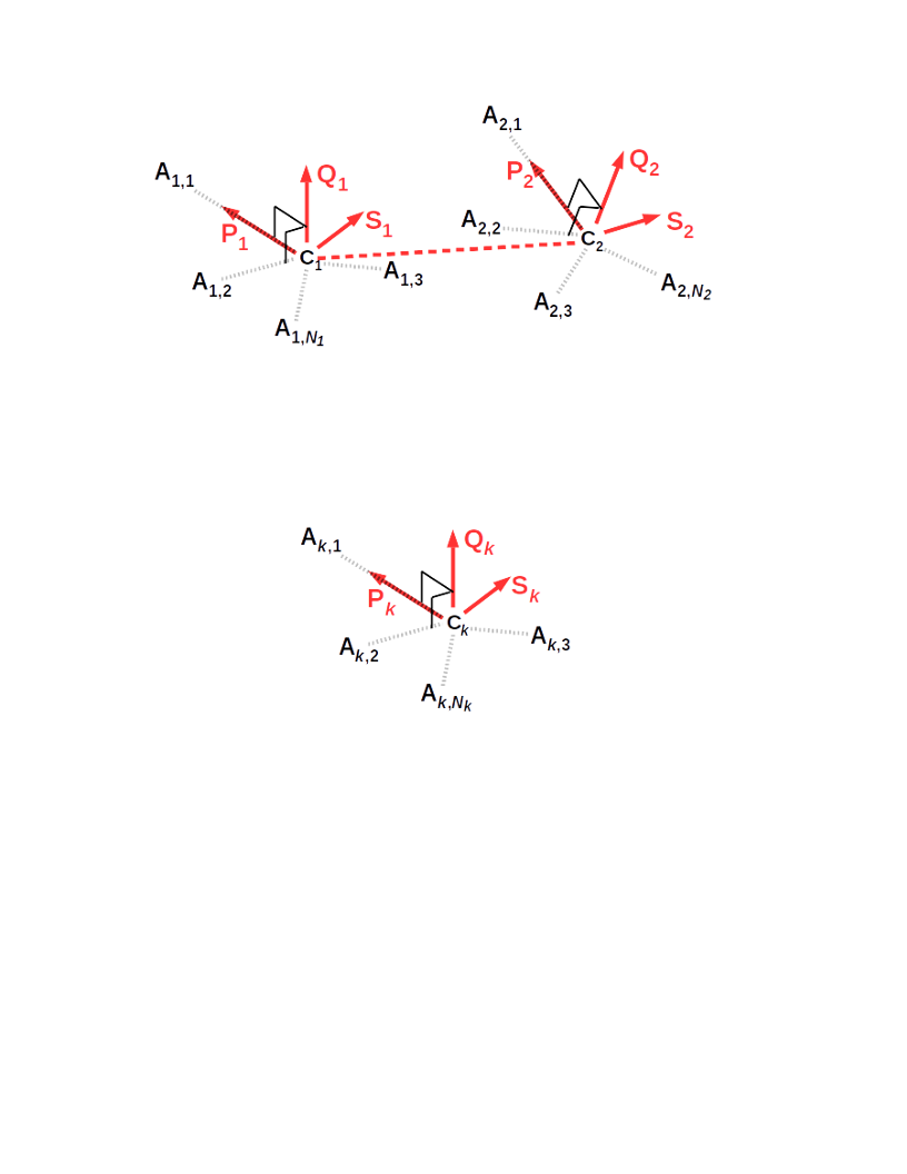
Rotor(Label1,Label2)
Replace the current GICs that describe the motion of the fragments Label1 and Label2 relative to each other and the remaining fragments with a special set of rotational and translational GICs (see above). Then express them in terms of the dot products:
ΔC1·P2, ΔC1·Q2, ΔC1·S2,
ΔC2·P1, ΔC2·Q1, ΔC2·S1,
P1·P2, Q1·P2, S1·P2,
P1·Q2, Q1·Q2, S1·Q2,
P1·S2, Q1·S2, S1·S2
where ΔC1 = C1 – C2, ΔC2 = C2 – C1, Ck = (Cxk,Cyk,Czk), Pk = (Pxk,Pyk,Pzk), Qk = (Qxk,Qyk,Qzk), Sk = (Sxk,Syk,Szk), and k = 1 refers to the fragment Label1 and k = 2 refers to the fragment Label2. The vector Ck defines the position of the geometric center of the corresponding fragment with respect to the origin of Cartesian coordinates. The user should specify the fragments explicitly along with their labels using the Fragment() specification prior to executing this option. If there are no user-provided fragments then the program will attempt to assign the default fragments (labeled by default as FRGM1, FRGM2, etc.) using the current connectivity data based on the input Cartesian geometry, if possible. To find some input examples that use this option, run the following command:
grep -i 'Rotor(' $gdvroot/gdv/tests/com/*.com | grep -e ','
List of available mathematical operations
Unary operations
The available unary operations described below operate on an argument A which can be the label of a previously defined coordinate or a valid GIC symbolic expression including an integer or floating-point number.
SQRT(A)
Take the square root of an argument.
EXP(A)
Take the exponent of an argument, i.e., eA.
SIN(A)
Take the sine of an argument.
COS(A)
Take the cosine of an argument.
TAN(A)
Take the tangent of an argument.
ARCSIN(A)
Take the inverse sine of an argument or arcsine.
ARCCOS(A)
Take the inverse cosine of an argument or arccosine.
ARCTAN(A)
Take the inverse tangent of an argument or arctangent.
Binary operations
The available binary operations described below operate on the arguments A and B which can be the labels of previously defined coordinates or any valid GIC symbolic expressions that involve integer or floating-point numbers.
A+B
Addition of two arguments.
A–B
Subtraction of two arguments.
A*B
Multiplication of two arguments.
A/B
Division of argument A by argument B.
Other operations
A**N
Take the N-th power of an argument. The base A can be the label of a previously defined coordinate or a valid GIC symbolic expression. The exponent N is an integer. Synonyms: A^N.
ATAN2(Y,X)
Take the two-argument arctangent where X and Y are the labels of two previously defined coordinates or valid GIC symbolic expressions. The atan2(Y,X) function is equal to the angle θ defined in radians as −π < θ ≤ π where X = R * cos(θ), Y = R * sin(θ), and R =
Options given with the coordinate’s label or expression
The word “Options” refers to one or more GIC-related keywords separated by commas in the case of “Label(Options)” format or by spaces in the case of the “Expression Options” format. In particular, one of the keywords can be the coordinate’s action flag having one of the following (case-insensitive) values. Replace “Label” with the coordinate’s actual label and replace “Expression” with the actual expression (with no quotation marks).
Active
Build a new coordinate defined by the given expression with an optional user-provided label and flag it as active and unfrozen (i.e., add it to the list of internal coordinates used in geometry optimization and let its value change during the optimization). If the given expression or the coordinate’s label has been previously added as inactive or frozen, then flag the coordinate as active and unfrozen. Note that this option is similar to the option A used in the ModRedundant input section with Geom=ModRedundant (now Geom=(DefNoGIC,ModRedundant) for the old algorithm (Peng96)). Synonyms: Activate, Add. This flag is default.
Frozen
Build a coordinate defined by the expression (with an optional user-provided label) if it does not exist, flag the coordinate active for geometry optimization and freeze it at the current value. Note that this option is similar to the option F used in the ModRedundant input section for the old algorithm (Peng96). Synonyms: Freeze.
Remove
(1) Build a new coordinate defined by the expression (with an optional user-provided label) and flag it inactive (i.e., do not include it in geometry optimization), or (2) if the coordinate with the given label or for the given expression has been already built and flagged as active frozen or active unfrozen then remove it from the geometry optimization by flagging it as inactive. Note that this option is similar to the option R used in the ModRedundant input section for the old algorithm (Peng96). Synonyms: Inactive.
RemoveAll
Remove the coordinate from the list of internal coordinates used in geometry optimization along with any dependent coordinates by flagging all of them as inactive. The dependent coordinates include any coordinate that depends on the same atoms as the given coordinate. For example, “R(1,5) RemoveAll” will result in removing the coordinate R(1,5) referring to the internuclear distance between atom 1 and atom 5 as well as the valence angles, dihedral angles, or any arbitrary coordinate that depend on the Cartesian coordinates of atoms 1 and 5 in combination with any other atoms in the molecule. Note that this option is similar to the option K used in the ModRedundant input section for the old algorithm (Peng96).
PrintOnly
Print a current value of the coordinate defined by the expression with the label but do not add the coordinate to the list of internal coordinates used in geometry optimization. The proper use of this flag is “Label(PrintOnly)=Expression” or “Label(PrintOnly)” if the expression has been already defined. Note that the user can also specify IOp(1/33=1) to print the initial and current values of all the GICs with labels (including the GICs used as intermediate expressions in the user-provided GIC input section) without using the PrintOnly option.
Modify
In the case of the “Label(Options)=Expression” format only, replace the old coordinate known by the label “Label” with the new expression and flag the newly modified coordinate as active and unfrozen.
FlBon
Treat the coordinate as a regular bond when it matters and print the value in Angstroms by default. Note this expression as an example:
distAzBz(FlBon)=sqrt[(x(13)-xAz)^2+(y(13)-yAz)^2+(z(13)-zAz)^2]
FlAng
Treat the coordinate as a regular valence angle when it matters, print the value in degrees by default, and assume that it changes from 0º to 180º. Note these expressions as an example:
A1b(FlAng)=ARCCOS((Qx1*(X(4)-X(1))+Qy1*(Y(4)-Y(1))+Qz1*(Z(4)-Z(1)))/R(1,4)/RQ1)
A214a(FlAng)=ATAN2(YH2,XH2)
FlDih
Treat the coordinate as a dihedral angle when it matters, print the value in degrees by default, and assume that it changes from −180º to 180º.
FlPQS
Treat the coordinate as one of the Cartesian components of a rotational unit vector (Px, Py, …, Sz) or the quaternion vector components (K1, K2, or K3) and assume that it changes between −1 and +1 in atomic units. Note these expressions as an example:
K1F1(FlPQS)=(Qz1-Sy1)/(4*K0F1)
K2F1(FlPQS)=(Sx1-Pz1)/(4*K0F1)
K3F1(FlPQS)=(Py1-Qx1)/(4*K0F1)
FlQua0
Treat the coordinate as the scalar quaternion component (K0) and assume that it changes between 0 and +1 in atomic units. Note this expression as an example:
K0F1(FlQua0)=0.5*Sqrt(Px1+Qy1+Sz1+1)
Diff
Calculate numerical second derivatives for the row and column of the initial Hessian for this coordinate. Note that this option is similar to the option D used in the ModRedundant input section for the old algorithm (Peng96).
Note that in the case of the “Expression Options” format, the flags Active, Diff, Frozen, Remove, and RemoveAll can be replaced with a single letter A, D, F, R, and K, respectively.
FC=X
Change the diagonal element for the coordinate in the initial Hessian to X where X is a floating-point value in atomic units. Note that this option is similar to the option H used in the ModRedundant input section for the old algorithm (Peng96). Synonyms: ForceConstant.
Value=X
Set an initial value for the given internal coordinate to X where X is a floating-point value in the units defined by the Units keyword (Angstroms or degrees by default). The current Cartesian coordinates will be adjusted to match this value as closely as possible. This option should be used cautiously and sparingly. It is far easier and more reliable to set the initial molecular structure as desired in a graphic environment like GaussView.
StepSize=X,NSteps=N
Perform a relaxed potential energy surface scan. Increment the coordinate N times by the step X where X is a floating-point value in the units defined by the Units keyword (Angstroms or degrees by default). In the case of the “Expression Options” format, the comma between the keywords can be replaced with a space.
Min=XMn,Max=XMx
Add, freeze, or remove the coordinate if during the geometry optimization its value X satisfies the XMn<=X<=XMx relation where XMn and XMx are user-provided floating-point values in the units defined by the Units keyword (Angstroms or degrees by default). If there is no Min=XMn given, the condition reduces to X<=XMx. If there is no Max=XMx given, the condition reduces to XMn<=X. The Min/Max option can only be used in combination with the flags Active, Frozen, or Remove. In the case of the “Expression Options” format, the comma between the keywords can be replaced with a space. Some examples of using these options can be found by running the following command:
grep -i -e 'Min=' -e 'Max=' $gdvroot/gdv/tests/com/*.com
There are two more keywords that can be used along with the coordinate’s expression.
Expression Flag OnlyIf Expression2
Add, freeze, or remove a coordinate defined by “Expression” only if another (previously introduced) coordinate defined by “Expression2” is included in the geometry optimization. The word “Flag” should be replaced with the flags Active, Frozen, or Remove to add, freeze, or remove, respectively. The words “Expression” and “Expression2” should be replaced with mathematical expressions (without the “=” signs) or with the coordinates’ labels if the latter are known. The keyword OnlyIf is not case sensitive but should be spelled as one word.
Expression Flag IfNot Expression2
Add, freeze, or remove a coordinate defined by “Expression” only if another (previously introduced) coordinate defined by “Expression2” is not included in the geometry optimization. The word “Flag” should be replaced with the flags Active, Frozen, or Remove (or with their synonyms) to add, freeze, or remove, respectively. The words “Expression” and “Expression2” should be replaced with mathematical expressions (without the “=” signs) or with the coordinates’ labels if the latter are known. The keyword IfNot is not case sensitive but should be spelled as one word.
Standalone options
There are several options that can be used without the coordinate’s label or expression and they serve as global instructions.
FreezeAll
Freeze any internal coordinate previously added as active to the list of coordinates used in geometry optimization.
UnFreezeAll
Unfreeze any internal coordinate previously added as active frozen to the list of coordinates used in geometry optimization.
RemoveAll
Remove any internal coordinate previously added as active frozen and active unfrozen from the list of coordinates used in geometry optimization.
Atom i
Add the Cartesian coordinates of atom i to the list of internal coordinates used for geometry optimization. If the integer i is replaced with the wildcard symbol “*” then add the Cartesian coordinates of all atoms.
Atom i Freeze
Add the Cartesian coordinates of atom i to the list of internal coordinates used for geometry optimization and freeze them at their initial values.
Atom i UnFreeze
Unfreeze the Cartesian coordinates of atom i previously added to the list of internal coordinates as frozen.
Atom i Remove
Remove the previously added Cartesian coordinates of atom i from the list of internal coordinates used for geometry optimization.
Atom i RemoveAll
Remove the Cartesian coordinates of atom i from the list of internal coordinates used for geometry optimization and also remove any other internal coordinate that depends on atom i.
Atom i XYZOnly
Remove any internal coordinate that depends on atom i from the list of coordinates used for geometry optimization but add or keep the Cartesian coordinates of that atom.
RdOpt
There may be situations when certain atoms need to be frozen in terms of their Cartesian coordinates while keeping the internal coordinates connecting those atoms to the remaining ones unfrozen. Here is an example how to proceed in such a case:
#p HF/STO-3G Opt=(RdOpt,GIC)

Test 1

0 1
 C                 -0.08857879    0.12689103    0.00000000
 O                 -0.62172704    1.20626440    0.00000000
 O                 -0.79640759   -1.03149748    0.00000000
 H                 -1.73495142   -0.78582182    0.00000000
 C                  1.39215704   -0.12787100    0.00000000
 H                  1.56703747   -0.91337923    0.89935717
 H                  1.56703747   -0.91337923   -0.89935717
 H                  1.92446969    0.81936763    0.00000000

notatoms=1-4
In this example, the default GICs over all the atoms are modified by replacing the internal coordinates interconnecting the atoms 1, 2, 3, and 4 (which need to be frozen) with the frozen Cartesian coordinates of those atoms while keeping the remaining GICs as is. The latter include the GICs over the remaining (unfrozen) atoms and the GICs connecting the frozen atoms to the unfrozen ones. Here is another way to freeze the atoms:
#p HF/STO-3G Opt=GIC

Test 1

0 1
 C     -1        -0.08857879    0.12689103    0.00000000
 O     -1        -0.62172704    1.20626440    0.00000000
 O     -1        -0.79640759   -1.03149748    0.00000000
 H     -1        -1.73495142   -0.78582182    0.00000000
 C                1.39215704   -0.12787100    0.00000000
 H                1.56703747   -0.91337923    0.89935717
 H                1.56703747   -0.91337923   -0.89935717
 H                1.92446969    0.81936763    0.00000000
Use of some miscellaneous options and flags (HR, GicPhase, and GicStep)
The HR flag and the corresponding input data (explained and used elsewhere outside the GIC code) can be introduced via a GIC input section as follows:
#p HF/3-21G Geom=(Connectivity,ReadAllGic) IOp(1/33=3) Test

Gaussian Test Job XXXX (Part 1):
Testing the input for additional parameters with the HR flag and
CrdPa1 to extract them from CrData; look for HR Parameters in the output

0 1
 O                  0.00000000    0.00000000   -0.11081188
 H                  0.00000000   -0.78397589    0.44324751
 H                 -0.00000000    0.78397589    0.44324751

 1 2 1.0 3 1.0
 2
 3

 ROH1=R(1,2)
 ROH2=R(1,3)
 AHOH(HR,IVars=2,RVars1=0.1,RVars2=0.12,RVars3=0.123)=A(2,1,3)
An example of using this option can be found by running the following command:
grep -i '(HR=' $gdvroot/gdv/tests/com/*.com
There is also an experimental option called GicPhase to explicitly specify the period of a periodic GIC. For example, any pure dihedral angle should have GicPhase=2π which is trivial and is determined by default. For a more complicated periodic GIC, the GicPhase value is also determined by default when needed but the option can be used for debugging. See IOp(1/155=nxxxxxx) for more detail. There is another experimental option called GicStep to explicitly specify the maximum displacement allowed for a particular GIC when making an optimization step. Examples of using these two options can be found by running the following command:
grep -i -e 'gicphase' -e 'gicstep' $gdvroot/gdv/tests/com/*.com
Use of the old ModRedundant format
Modifications to the GICs can be read in by using the ModRedundant format from the old internal coordinate algorithm available in Gaussian 16. See the ModRedundant section in the G16 reference for the Opt keyword. However, the old format is available only for the GICs that are pure bonds, angles, or torsions (dihedral angles). In addition, the old format and the new GIC format described above cannot be mixed together in the same input section.
Note about the default GIC labels and units in Gaussian output
The summary of generated GICs and their initial values is printed in the “Initial Parameters” table in the Gaussian output from any calculation that uses such GICs (see some examples below). The column “Name” contains the short labels and the column “Definition” contains the long labels. The default set of coordinates may include regular valence bonds, valence or linear angles, and dihedral angles. The default short labels for the bonds are R1, R2, …, Rn where n runs over all generated bonds in the order of appearance. The default short labels for valence or linear angles are A1, A2, A3, etc. The default labels for dihedral angles are D1, D2, D3, etc. The long (definition) labels for the bonds, valence angles, and dihedral angles are printed (for example) as R(1,2), A(2,1,3), and D(2,1,3,4) in terms of the corresponding atomic indexes for atoms 1, 2, 3, and 4. The definition label of a two-component linear bend (defined earlier) includes five indexes, and can be L(1,2,3,4,-1) or L(1,2,3,4,-2) for example.
The default set of coordinates may include XY3-type GICs for suitable XY3 groups and PQS-type GICs for geometries with fragments. Those coordinates are generic GICs in the sense that they are not pure bonds, valence angles, and dihedral angles. The default labeling for those GICs is explained earlier in this document. Note that their definitions are not printed by default and the long (definition) label for each generic coordinate reduces to “GIC-i” (for simplicity) where i is the index of a primitive GIC associated with the corresponding coordinate. The whole symbolic algebra tree can be printed out by using Geom=GICPrint.
The values of the GICs defined as pure distances, valence angles or linear bends, and dihedral angles or torsions are computed from the Cartesian coordinates in atomic units (Bohrs) and stored internally in Bohrs and radians (respectively, for distances and angles) but, for the user’s convenience, they are printed out in Angstroms (Å) and degrees (see, for example, the “Initial Parameters” table). In the case of a generic GIC, the GIC value is computed as a function of Cartesian coordinates in Bohrs, bond distances in Bohrs, and/or valence, linear or dihedral angles in radians combined with optional constants (e.g., weights or scale factors) in user-defined units. Such generic GIC values (labeled as “GIC”) are computed, stored and printed in the same units which are procedure-defined or arbitrary units in general. If the GIC is a combination of bonds or a combination of valence angles scaled with dimensionless weight factors then the arbitrary units become Bohrs for the bonds and radians for the angles.
Further examples of using GICs
Basic GIC input and output.
Here is an example of using the generalized internal coordinates defined by the user from scratch for the geometry optimization of the water molecule.
# HF opt=ReadAllGIC

Title

0 1
O    0.0000    0.0000    0.0000
H    0.0000    0.0000    1.3112
H    1.0354    0.0000   -0.6225

R(1,2)
R(1,3)
HOH=A(2,1,3)
The atomic indexes 1, 2, and 3 refer to the oxygen atom, the first and the second hydrogen atom, respectively. The first and the second expression define the O-H bonds, and the third one defines the H-O-H valence angle (with the user-provided label “HOH”). An excerpt of the output with a table containing the initial values of the GICs is shown below.
                            ----------------------------
                           !    Initial Parameters     !
                           ! (Angstroms and Degrees)   !
--------------------------                            --------------------------
! Name  Definition              Value          Derivative Info.                !
--------------------------------------------------------------------------------
! R1    R(1,2)                  1.3112         estimate D2E/DX2                !
! R2    R(1,3)                  1.2081         estimate D2E/DX2                !
! HOH   A(2,1,3)              121.015         estimate D2E/DX2                !
--------------------------------------------------------------------------------
Note that the labels “R1” and “R2” above were assigned by default. The coordinates R1=R(1,2) and R2=R(1,3) are parsed as pure distances and given here in Angstroms, and the HOH=A(2,1,3) is a pure valence angle in degrees.
# HF opt=ReadAllGIC

Title

0 1
O    0.0000    0.0000    0.0000
H    0.0000    0.0000    1.3112
H    1.0354    0.0000   -0.6225

OHSym1=(R(1,2)+R(1,3))/sqrt(2)
OHSym2=(R(1,2)-R(1,3))/sqrt(2)
HOH=A(2,1,3)
The first and the second expression in the example above define the symmetrized O-H bonds, and the third one is the H-O-H valence angle.
                            ----------------------------
                           !    Initial Parameters     !
                           ! (Angstroms and Degrees)   !
--------------------------                            --------------------------
! Name   Definition             Value          Derivative Info.                !
--------------------------------------------------------------------------------
! OHSym1 GIC-9                  3.3664         estimate D2E/DX2                !
! OHSym2 GIC-11                 0.1377         estimate D2E/DX2                !
! HOH    A(2,1,3)             121.015         estimate D2E/DX2                !
--------------------------------------------------------------------------------
NOTE: GIC-type coordinates are in arbitrary units.
The coordinates OHSym1 and OHSym2 are parsed as generic GICs and therefore given here in arbitrary units. The units are actually Bohrs in this case because the 2-1/2 factor is taken as dimensionless and the values of R(1,2) and R(1,3) are taken in Bohrs.
# HF opt=ReadAllGIC

Title

0 1
O
H  1  1.3
H  1  1.2  2  120.

R12=SQRT[{X(2)-X(1)}^2+{Y(2)-Y(1)}^2+{Z(2)-Z(1)}^2]
R13=SQRT[{X(3)-X(1)}^2+{Y(3)-Y(1)}^2+{Z(3)-Z(1)}^2]
A0(Inactive)=DotDiff(2,1,3,1)/{R12*R13}
A213=ArcCos(A0)
The GIC input section above defines two bond distances and one valence angle expressed via Cartesian coordinates as generic GICs. The coordinate A0 is defined as the dot product (DotDiff) of the vectors and divided by the product of their lengths, and it is selected as “inactive” (i.e., excluded from the geometry optimization). An excerpt of the output with a table containing the initial values of those GICs is shown below.
                            ----------------------------
                           !    Initial Parameters     !
                           ! (Angstroms and Degrees)   !
--------------------------                            --------------------------
! Name  Definition              Value          Derivative Info.                !
--------------------------------------------------------------------------------
! R12   GIC-15                  2.4566         estimate D2E/DX2                !
! R13   GIC-27                  2.2677         estimate D2E/DX2                !
! A213  GIC-31                  2.0944         estimate D2E/DX2                !
--------------------------------------------------------------------------------
NOTE: GIC-type coordinates are in arbitrary units.
The values of R12, R13, and the dot product are calculated using the Cartesian coordinates given in Bohrs. The GIC arbitrary units are Bohrs (for R12 and R13) and radians (for A213). Note that the integer i in the definition label for any generic GIC (“GIC-i“) refers to the index of a primitive GIC associated with the corresponding coordinate. The whole symbolic algebra tree can be printed out by using Geom=GICPrint.
ModRedundant Input Syntax
Lines in a ModRedundant input section use the following syntax:
[Type] N1 [N2 [N3 [N4]]] [A | F]
[Type] N1 [N2 [N3 [N4]]] B
[Type] N1 [N2 [N3 [N4]]] K | R
[Type] N1 [N2 [N3 [N4]]] D
[Type] N1 [N2 [N3 [N4]]] H diag-elem
[Type] N1 [N2 [N3 [N4]]] S nsteps stepsize
N1, N2, N3, and N4 are atom numbers or wildcards (discussed below). Atom numbering begins at 1, and any dummy atoms are not counted.
The atom numbers are followed by a one-character code letter indicating the coordinate modification to be performed; the action code is sometimes followed by additional required parameters as indicated above. If no action code is included, the default action is to add the specified coordinate. These are the available action codes:
| A | Activate the coordinate for optimization if it has been frozen. |
| F | Freeze the coordinate in the optimization. |
| B | Add the coordinate and build all related coordinates. |
| K | Remove the coordinate and kill all related coordinates containing this coordinate. |
| R | Remove the coordinate from the definition list (but not the related coordinates). |
| D | Calculate numerical second derivatives for the row and column of the initial Hessian for this coordinate. |
| H | Change the diagonal element for this coordinate in the initial Hessian to diag-elem. |
| S | Perform a relaxed potential energy surface scan. Increment the coordinate by stepsize a total of nsteps times, performing an optimization from each resulting starting geometry. |
An asterisk (*) in the place of an atom number indicates a wildcard. Here are some examples of wildcard use:
| * | All atoms specified by Cartesian coordinates. |
| * * | All defined bonds. |
| 3 * | All defined bonds with atom 3. |
| * * * | All defined valence angles. |
| * 4 * | All defined valence angles around atom 4. |
| * * * * | All defined dihedral angles. |
| * 3 4 * | All defined dihedral angles around the bond connecting atoms 3 and 4. |
By default, the coordinate type is determined from the number of atoms specified: Cartesian coordinates for 1 atom, bond stretch for 2 atoms, valence angle for 3 atoms, and dihedral angle for 4 atoms. Optionally, type can be used to designate these and additional coordinate types:
| X | Cartesian coordinates. |
| B | Bond length. |
| A | Valence angle. |
| D | Dihedral angle. |
| L | Linear bend specified by three atoms (if N4 is -1) or by four atoms, where the fourth atom is used to determine the 2 orthogonal directions of the linear bend. |
Examples
Modifying Redundant Internal Coordinates. The following input file illustrates the method for modifying redundant internal coordinates within an input file:
| # HF/6-31G(d) Opt=ModRedun Test | |
| Opt job | |
| 0,1 | |
| C1 0.000 0.000 0.000 | |
| C2 0.000 0.000 1.505 | |
| O3 1.047 0.000 -0.651 | |
| H4 -1.000 -0.006 -0.484 | |
| H5 -0.735 0.755 1.898 | |
| H6 -0.295 -1.024 1.866 | |
| O7 1.242 0.364 2.065 | |
| H8 1.938 -0.001 1.499 | |
| 3 8 | Adds hydrogen bond (but not angles or dihedrals). |
| 2 1 3 | Adds C-C-O angle. |
This structure is acetaldehyde with an OH substituted for one of the hydrogens in the methyl group; the first input line for ModRedundant creates a hydrogen bond between that hydrogen atom and the oxygen atom in the carbonyl group. Note that this adds only the bond between these two atoms The associated angles and dihedral angles could be added as well using the B action code:
3 8 B
Displaying the Value of a Desired Coordinate. The second input line for ModRedundant specifies the C-C=O bond angle, ensuring that its value will be displayed in the summary structure table for each optimization step.
Using Wildcards in Redundant Internal Coordinates. A distance matrix coordinate system can be activated using the following input:
| * * B | Define all bonds between pairs of atoms |
| * * * K | Remove all other redundant internal coordinates |
The following input defines partial distance matrix coordinates to connect only the closest layers of atoms:
| * * B 1.1 | Define all bonds between atoms within 1.1 Å |
| * * * K | Remove all other redundant internal coordinates |
The following input sets up an optimization in redundant internal coordinates in which atoms N1 through Nn are frozen (such jobs may require the NoSymm keyword). Note that the lines containing the B action code will generate Cartesian coordinates for all of the coordinates involving the specified atom since only one atom number is specified:
| N1 B | Generate Cartesian coordinates involving atom N1 |
| … | |
| Nn B | Generate Cartesian coordinates involving atom Nn |
| * F | Freeze all Cartesian coordinates |
The following input defines special “spherical” internal coordinates appropriate for molecules like C60 by removing all dihedral angles from the redundant internal coordinates:
| * * * * R | Remove all dihedral angles |
Additional examples are found in the section on relaxed PES scans below.